Random Variable and Mathematical Expectation Exercise 6.1

Dear Class 12 Samacheer Kalvi students, here are the Text Book Solutions for Exercise 6.1 Business Maths Chapter 6 Random Variable and Mathematical for your reference and study.

You can find links to the other exercises below.

Important Formulas in Random Variable and Mathematical Expectation

Text Book Solutions for Differential Equations Exercise 6.2

Text Book Solutions for Differential Equations Exercise 6.3

Exercise 6.1

$1.\;\text{Construct cumulative distribution function for the given probability distribution.} \\$

X	0	1	2	3
P(X=x)	0.3	0.2	0.4	0.1

$F(x)=P(X=x) \\$
$F(0)=P(X\le 0) \;= P(0)\; =0.3 \\$
$F(1)=P(X\le 1) \\$
$F(1)=P(0)+P(1)\; =0.3+0.2\;=0.5 \\$
$F(2)=P(X\le 2) \\$
$F(2)=P(0)+P(1)+P(2)\; =0.3+0.2+0.4\;=0.9 \\$
$F(3)=P(X\le 3) \\$
$F(3)=P(0)+P(1)+P(2)+P(3)\; =0.3+0.2+0.4+0.1\;=1 \\$

X	0	1	2	3
P(X=x)	0.3	0.5	0.9	1

$2.\; \text{Let X be a discrete random variable with the following p.m.f} \\$
$p(x) = \begin{cases} & 0.3 \; \text{ for x=3 } \\ & 0.2 \; \text{ for x=5 } \\ & 0.3 \; \text{ for x=8 } \\ & 0.2 \; \text{ for x=10 } \\ & 0 \text{ otherwise} \end{cases} \\$
$\text{Find and plot the c.d.f. of X .} \\$

X	3	5	8	10
P(x)	0.3	0.2	0.3	0.2

$F(x)=P(X\le x) \\$
$F(3)=P(X\le 3) \;= p(3)\; =0.3 \\$
$F(5)=P(X\le 5) \\$
$F(5)=P(3)+P(5)\; =0.3+0.2\;=0.5 \\$
$F(8)=P(X\le 8) \\$
$F(8)=P(3)+P(5)+P(8)\; =0.3+0.2+0.3\;=0.8 \\$
$F(10)=P(X\le 10) \\$
$F(10)=P(3)+P(5)+P(8)+P(10)\; =0.3+0.2+0.3+0.2\;=1 \\$

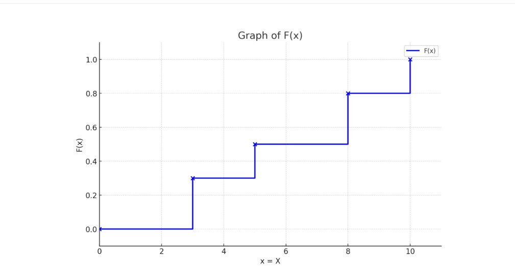
X	3	5	8	10
P(x)	0.3	0.5	0.8	1

$F(x) = \begin{cases} & 0 \; \text{ for } x < 3 \\ & 0.3 \; \text{ for}\;3\le x < 5 \\ & 0.5 \; \text{ for}\;5\le x < 8 \\ & 0.8 \; \text{ for }\;8\le x < 10 \\ & 1 \text{ for}\; x > 10 \end{cases}\\$

Graph of F(x)

$3.\; \text{The discrete random variable X has the following probability function} \\$
$P(X=x) \begin{cases} & kx \hspace{20 mm} x=2,4,6 \\ & k(x-2) \hspace{10 mm} x=8 \\ & 0 \text{ otherwise} \end{cases}$
$\text{where k is a constant. Show that}\; k=\displaystyle \frac{1}{18}. \\$

X	2	4	6	8
P(x)	2k	4k	6k	6k

Since p(x) is p.m.f

$\sum_{}^{}p(x)=1 \\$
$p(2)+p(4)+p(6)+p(8)=1 \\$
$2k+4k+6k+6k=1 \\$
$18k=1 \\$
$k=\frac{1}{18} \\$
$\text {Proved.} \\$

$4.\; \text{The discrete random variable X has the probability function} \\$

X	1	2	3	4
P(x)	k	2k	3k	4k

$\text{Show that k = 0⋅1} \\$

Since p(x) is p.m.f

$\sum_{}^{}p(x)=1 \\$
$p(1)+p(2)+p(3)+p(4)=1 \\$
$k+2k+3k+4k=1 \\$
$10k=1 \\$
$k=\frac{1}{10} \\$
$\text {Proved.} \\$

$5.\;\text{5. Two coins are tossed simultaneously. Getting a head is termed as success.} \\$
$\text{Find the probability distribution of the number of successes.} \\$

$\text{Let X be the event of getting heads.} \\$
$X=0,1,2 \\$
$Sample Space = {HH, HT,TH,TT} \\$
$p(0)=\frac{1}{4} \\$
$p(1)=\frac{2}{4} \; \frac{1}{2}\\$
$p(2)=\frac{1}{4} \\$

X	0	1	2
P(x)	1/4	1/2	1/4

$6.\; \text{A continuous random variable X has the following probability function} \\$

Value of X=x	0	1	2	3	4	5	6	7
p(x)	0	k	2k	2k	3k	k²	2k²	7k² +k

$(i) \;\text{Find k} \\$
$(ii)\;\text{Evaluate}\; p( x < 6),\; p(x \ge 6)\;\text{and}\; p(0 < x < 5) \\$
$(iii)\;\text{If}\;P(X\le x) > \displaystyle \frac{1}{2} \\$
$\text {then find the minimum value of x.} \\$

$\text{Since p(x) is p.m.f} \\$
$\sum_{}^{}p=1 \\$
$\text{p(0)+p(1)+p(2)+p(3)+p(4)+p(5)+p(6)+p(7)}=1 \\$
$0+k+2k+2k+3k+k^{2}+2k^{2}+7k^{2}+k=1 \\$
$10k^{2}+9k-1=0 \\$
$10k^{2}+10k-k-1=0 \\$
$10k(k+1)-1(k+1)=0 \\$
$(10k-1)k+1)=0 \\$
$\begin{array}{c|c} 10k-1=0 & k+1=0\\ 10k=1 & k=-1 \\ k=\displaystyle \frac{1}{10}& k=-1 \\ \end{array}\\$
$k=-1 \;\text{is not possible}\\$
$\text{Therefore} \; k=\displaystyle \frac{1}{10}\\$

$(ii)\;p(x > 6)=p(0)+p(1)+p(2)+p(3)+p(4)+p(5) \\$
$0+k+2k+2k+3k+k^{2} \\$
$k^{2}+8k \\$
$\left( \displaystyle \frac{1}{10} \right)^{2}+8\left( \displaystyle \frac{1}{10} \right)\\$
$\displaystyle \frac{1}{100} + \displaystyle \frac{8}{10} \\$
$\displaystyle \frac{1+80}{100}\\$
$p(x > 6)=\displaystyle \frac{81}{100}\\$

$\;p(x\ge 6)=p(6)+p(7)\\$
$2k^{2} +7k^{2}+k\\$
$9k^{2}+k \\$
$9 \left(\displaystyle \frac{1}{10} \right)^{2}+\left( \displaystyle \frac{1}{10} \right)\\$
$9\left( \displaystyle \frac{1}{100} \right)+\displaystyle \frac{1}{10}\\$
$\displaystyle \frac{9}{100}+\displaystyle \frac{1}{10}\\$
$\displaystyle \frac{9+10}{100}\\$
$p(x \ge 6)=\displaystyle \frac{19}{100}\\$

$p(0< x< 5)=p(1)+p(2)+p(3)+p(4) \\$
$k+2k+2k+3k\\$
$8k\\$
$8\times\displaystyle \frac{1}{10}\\$
$p(0< x< 5)=\displaystyle \frac{8}{10}\\$

$(iii)\; p(x\le 0)=p(0)=0< \displaystyle \frac{1}{2} \\$
$p(x\le 1)=p(0)+p(1) \\$
$=0+k=k \\$
$=\displaystyle \frac{1}{10}< \displaystyle \frac{1}{2} \\$
$p(x\le 2)=p(0)+p(1)+p(2) \\$
$=0+k+2k=3k \\$
$=3\times \displaystyle \frac{1}{10}\\$
$=\displaystyle \frac{3}{10}< \displaystyle \frac{1}{2}\\$
$p(x\le 3)=p(0)+p(1)+p(2)+p(3)\\$
$=0+k+2k+2k=5k\\$
$=5\times \displaystyle \frac{1}{10}\\$
$=\displaystyle \frac{5}{10}= \displaystyle \frac{1}{2}\\$
$p(x\le 4)=p(0)+p(1)+p(2)+p(3)+p(4)\\$
$=0+k+2k+2k+3k=8k\\$
$=8\times \displaystyle \frac{1}{10}\\$
$=\displaystyle \frac{8}{10} > \displaystyle \frac{1}{2}\\$
$\text{Therefore the value of x for }\;P(X\le x)> \displaystyle \frac{1}{2}=4\\$

$7. \;\text{The distribution of a continuous random variable X} \\$ $\text{in range (-3, 3) is given by p.d.f.} \\$
$f(x) = \begin{cases} & \frac{1}{16}(3+x)^{2} \hspace{10 mm} -3\le x\le -1 \\ & \frac{1}{16}(6-2x^{2})^{2} \hspace{5 mm} -1\le x\le 1 \\ & \frac{1}{16}(3-x)^{2} \hspace{12 mm} 1\le x\le 3 \end{cases} \\$
$\text {Verify that the area under the curve is unity.} \\$

$\displaystyle \int_{-3}^{3}f(x)\;dx=\displaystyle \int_{-3}^{-1}f(x)\;dx+\displaystyle \int_{-1}^{1}f(x)\;dx+\displaystyle \int_{1}^{3}f(x)\;dx \\$

$=\displaystyle \int_{-3}^{-1}\displaystyle \frac{1}{16}(3+x)^{2}\;dx+\displaystyle \int_{-1}^{1}\displaystyle \frac{1}{16}(16-2x^{2})\;dx+\displaystyle \int_{1}^{3}\displaystyle \frac{1}{16}(3-x)^{2}\;dx\\$

$=\displaystyle \frac{1}{16} \displaystyle \int_{-3}^{-1}(9+6x+x^{2})\;dx+\displaystyle \frac{1}{16} \displaystyle \int_{-1}^{1}(256-64x+4x^{2})\;dx+\displaystyle \frac{1}{16} \displaystyle \int_{1}^{3}(9-6x+x^{2})\;dx \\$

$=\displaystyle \frac{1}{16} \left[ 9+6x+x^{2} \right]_{-3}^{-1}+\displaystyle \frac{1}{16} \left[ 256-64x+4x^{2} \right]_{-1}^{1}+\displaystyle \frac{1}{16} \left[ 9-6x+x^{2} \right]_{1}^{3}\\$

$=\displaystyle \frac{1}{16} \Bigg[(-9-6+1)-(9-18+9)+ (256-64+4)-(256+64+4) +(9-18+9)-(9-6+1) \Bigg]\\$

$=1\\$
$\int_{-3}^{3}f(x)\;dx=1 \;\text{Verified}\\$

$8.\; \text{A continuous random variable X has the following distribution function} \\$
$F(x) = \begin{cases} & 0 \hspace{24 mm} if\; x \le 1 \\ & k(x-1)^{4} \hspace{5 mm} if\; 1 < x\le 3 \\ & 1 \hspace{24 mm} x > 3 \end{cases}\\$
$\text{Find (i) k and (ii) the probability density function.} \\$

$F(x) = \begin{cases} & 0 \hspace{24 mm} if\; x \le 1 \\ & k(x-1)^{4} \hspace{5 mm} if\; 1 < x\le 3 \\ & 1 \hspace{24 mm} x > 3 \end{cases}\\$
$f(x)=\displaystyle \frac{d\left( F(x) \right)}{dx}\\$
$f(x) = \begin{cases} & 0 \hspace{24 mm} if\; x \le 1 \\ & 4k(x-1)^{3} \hspace{5 mm} if\; 1 < x\le 3 \\ & 0 \hspace{24 mm} x > 3 \end{cases}\\$
$f(x) = \begin{cases} & 4k(x-1)^{3} \hspace{5 mm} if\; 1 < x\le 3 \\ & 0 \hspace{24 mm} otherwise \end{cases}\\$
$\text{(i)\; Since f(x) is p.d.f}\\$
$\displaystyle \int_{-\infty }^{\infty }f(x)=1\\$
$\displaystyle \int_{1 }^{3 }4k(x-1)^{3}\;dx=1 \\$
$4k \displaystyle \int_{1 }^{3 }(x-1)^{3}\;dx=1 \\$
$4k \displaystyle \int_{1 }^{3 }x^{3}-3x^{2}+3x-1\;dx=1 \\$
$4k\bigg[\frac{x^{4}}{4}-\frac{3x^{3}}{3}+\frac{3x^{2}}{2}-x\bigg]_{1}^{3}=1 \\$
$4k\bigg[\left( \frac{81}{4}-27+\frac{27}{2}-3 \right)- \bigg(\frac{1}{4}-1+\frac{3}{2}-1 \bigg)\bigg ] =1 \\$
$4k\bigg[\left( \frac{81}{4}+\frac{27}{2}-30 \right)- \bigg(\frac{1}{4}+\frac{3}{2}-2 \bigg)\bigg ] =1 \\$
$4k\bigg[\left( \frac{81+54-120}{4} \right)- \bigg(\frac{1+6-8}{4} \bigg)\bigg ] =1 \\$
$4k\bigg[\left( \frac{15}{4} \right)- \bigg(\frac{-1}{4} \bigg)\bigg ] =1 4k\bigg[\frac{16}{4}\bigg ] =1 \\$
$16k =1 \\$
$k=\displaystyle \frac{1}{16} \\$

$(ii)f(x) = \begin{cases} & 4k(x-1)^{3} \hspace{5 mm} if\; 1 < x\le 3 \\ & 0 \hspace{24 mm} otherwise \end{cases} \\$

$f(x) = \begin{cases} & 4\times\dfrac{1}{16}(x-1)^{3} \hspace{5 mm} if\; 1 < x\le 3 \\ & 0 \hspace{24 mm} otherwise \end{cases} \\$

$f(x) = \begin{cases} & \dfrac{1}{4}(x-1)^{3} \hspace{5 mm} if\; 1 < x\le 3 \\ & 0 \hspace{24 mm} otherwise \end{cases} \\$

$9.\; \text{The length of time (in minutes) that a certain person speaks on} \\$
$\text{the telephone is found to be random phenomenon, with a probability} \\$
$\text{function specified by the probability density function f (x) as} \\$
$f(x) = \begin{cases} & Ae^{\frac{-x}{5}} \hspace{14 mm} for\; x \ge 0 \\ & 0 \hspace{22 mm} otherwise \end{cases} \\$
$\text{(a) Find the value of A that makes f (x) a p.d.f.} \\$
$\text{(b) What is the probability that the number of minutes that person} \\$
$\text{ will talk over the phone is (i) more than 10 minutes,} \\$
$\text{(ii) less than 5 minutes and (iii) between 5 and 10 minutes.} \\$

$\text{a) Since f(x) is p.d.f} \\$
$\displaystyle \int_{-\infty}^{\infty}f(x)\;dx=1 \\$
$=\displaystyle \int_{0}^{\infty}Ae^{\dfrac{-x}{5}}\;dx=1 \\$
$=A\displaystyle \int_{0}^{\infty}e^{\dfrac{-x}{5}}\;dx=1 \\$
$=A \left( \dfrac{e^{\dfrac{-x}{5}}}{\dfrac{-1}{5}} \right)_{0}^{\infty}=1\\$
$= A \bigg(\dfrac{e^{\dfrac{-x}{5}}}{\dfrac{-1}{5}}\bigg)_{0}^{\infty}=1 \\$
$=-5A \bigg({e^{\dfrac{-x}{5}}} \bigg)_{0}^{\infty}=1 \\$
$= -5A \left( {e^{\dfrac{-\infty}{5}}} -{e^{\dfrac{0}{5}}} \right)=1 \\$
$=-5A \left( 0-1 \right)=1 \\$
$5A =1 \\$
$A=\dfrac{1}{5} \\$

$b.(i)\; p(x>10)=\displaystyle \int_{10}^{\infty}f(x)\;dx \\$
$\displaystyle \int_{10}^{\infty}Ae^{\dfrac{-x}{5}}\;dx \\$
$=A\displaystyle \int_{10}^{\infty}e^{\dfrac{-x}{5}}\;dx \\$
$=\dfrac{1}{5}\displaystyle \int_{10}^{\infty}\frac{e^{\dfrac{-x}{5}}}{\frac{-1}{5}}\;dx \\$

$=-1 \left( {e^{\dfrac{-x}{5}}} \right)_{10}^{\infty} \\$
$=-1 \left( {e^{\dfrac{-\infty}{5}}}-{e^{\dfrac{-10}{5}}} \right) \\$
$=-1 \left( 0-e^{-2} \right) \\$
$=e^{-2} \\$
$p(x>10)= \dfrac{1}{e^{2}}\\$

$(ii)\; p(x<5)=\displaystyle \int_{0}^{5}f(x)\;dx \\$
$\displaystyle \int_{0}^{5}Ae^{\dfrac{-x}{5}}\;dx \\$
$=A\displaystyle \int_{0}^{5}e^{\dfrac{-x}{5}}\;dx \\$
$=\dfrac{1}{5}\left[ \frac{e^{\dfrac{-x}{5}}}{\frac{-1}{5}} \right]_{0}^{5} \\$
$=-1 \left( {e^{\dfrac{-x}{5}}} \right)_{0}^{5} \\$

$=-1 \left( {e^{\dfrac{-5}{5}}}-{e^{\dfrac{0}{5}}} \right) \\$
$=-1 \left( e^{-1} -1\right) \\$
$=1-e^{-1} \\$
$=1-\dfrac{1}{e} \\$
$p(x < 5)= \dfrac{e-1}{e}\\$

$(iii)\; p(5 < x < 10)=\displaystyle \int_{5}^{10}f(x)\;dx \\$
$\displaystyle \int_{5}^{10}Ae^{\dfrac{-x}{5}}\;dx \\$
$=A\displaystyle \int_{5}^{10}e^{\dfrac{-x}{5}}\;dx \\$
$=\dfrac{1}{5}\left( \frac{e^{\dfrac{-x}{5}}}{\dfrac{-1}{5}} \right)_{5}^{10}\\$
$=-1 \left( {e^{\dfrac{-x}{5}}} \right)_{5}^{10} \\$
$=-1 \left( {e^{\dfrac{-10}{5}}}-{e^{\dfrac{-5}{5}}} \right)\\$

$=-1 \left( e^{-2} -e^{-1}\right)\\$
$=e^{-1} -e^{-2}\\$
$=\dfrac{1}{e} -\dfrac{1}{e^{2}}\\$
$p(5 < x < 10)= \dfrac{e-1}{e^{2}}\\$

$10.\; \text{Suppose that the time in minutes that a person has to wait }\\$
$\text{at a certain station for a train is found to be a random phenomenon }\\$
$\text{with a probability function specified by the distribution function}\\$
$\begin{equation} F(x) = \begin{cases} & 0 \hspace{24 mm} for\; x \le 0 \\ & \frac{x}{2} \hspace{20 mm} for\; 0\le x\le 1 \\ & \frac{1}{2} \hspace{20 mm} for\; 1\le x\le 2 \\ & \frac{x}{4} \hspace{20 mm} for\; 2\le x\le 4 \\ & 1 \hspace{24 mm} for \;x\ge 4 \end{cases}\\$
$\text{(a) Is the distribution function continuous? If so, give its} \\$
$\text{ probability density function?}\\$
$\text{(b) What is the probability that a person will have to wait }\\$ $\text{(i) more than 3 minutes,}\\$
$\text{(ii) less than 3 minutes and (iii) between 1 and 3 minutes?} \\$

$\text{a. Yes, the given distribution function is continuous.}}\\$
$\begin{equation} F(x) = \begin{cases} & 0 \hspace{24 mm} for\; x \le 0 \\ & \frac{x}{2} \hspace{20 mm} for\; 0\le x\le 1 \\ & \frac{1}{2} \hspace{20 mm} for\; 1\le x\le 2 \\ & \frac{x}{4} \hspace{20 mm} for\; 2\le x\le 4 \\ & 1 \hspace{24 mm} for \;x\ge 4 \end{cases}\\$
$f(x) = \dfrac{d(F(x))}{dx}= \begin{cases} & 0 \hspace{24 mm} for\; x \le 0 \\ & \frac{1}{2} \hspace{20 mm} for\; 0\le x\le 1 \\ & 0\hspace{20 mm} for\; 1\le x\le 2 \\ & \frac{1}{4} \hspace{20 mm} for\; 2\le x\le 4 \\ & 0 \hspace{24 mm} for \;x\ge 4 \end{cases}\\$
$f(x) = \begin{cases} & \frac{1}{2} \hspace{20 mm} for\; 0\le x\le 1 \\ & \frac{1}{4} \hspace{20 mm} for\; 2\le x\le 4 \\ & 0 \hspace{24 mm} otherwise \end{cases} \\$

$b.\; (i)\; p(x > 3)=\displaystyle \int_{3}^{4}f(x)\;dx \\$
$\displaystyle \int_{3}^{4}{\dfrac{1}{4}}\;dx \\$
${\dfrac{1}{4}} \displaystyle \int_{3}^{4}dx \\$
$=\dfrac{1}{4}\bigg( x \bigg)_{3}^{4}\\$
$=\dfrac{1}{4}(4-3)\\$
$=\dfrac{1}{4}\\$
$p(x > 3)= \dfrac{1}{4}\\$

$(ii)\; p(x < 3)=\displaystyle \int_{0}^{3}f(x)\;dx \\$
$\displaystyle \int_{0}^{1}f(x)\;dx +\displaystyle \int_{1}^{2}f(x)\;dx +\displaystyle \int_{2}^{3}f(x)\;dx\\$
$\displaystyle \int_{0}^{1}\dfrac{1}{2}\;dx +\displaystyle \int_{1}^{2}0\;dx \displaystyle \int_{2}^{3}\dfrac{1}{4}\;dx\\$
$\dfrac{1}{2}\displaystyle \int_{0}^{1}dx +0+ \dfrac{1}{4}\displaystyle \int_{2}^{3}dx\\$
$=\dfrac{1}{2}\bigg( x \bigg)_{0}^{1}+\dfrac{1}{4}\bigg( x \bigg)_{2}^{3}\\$
$=\dfrac{1}{2}\bigg(1-0\bigg)+\dfrac{1}{4}\bigg(3-2\bigg)\\$
$=\dfrac{1}{2}+\dfrac{1}{4}\\$
$=\dfrac{2+1}{4}\\$
$p(x < 3)=\dfrac{3}{4}\\$

$(iii)\; p(1 < x < 3)=\displaystyle \int_{1}^{3}f(x)\;dx \\$
$=\displaystyle \int_{1}^{3}x\;dx \\$
$=\displaystyle \int_{1}^{2}x\;dx +\displaystyle \int_{2}^{3}x\;dx \\$
$=\displaystyle \int_{1}^{2}0\;dx +\displaystyle \int_{2}^{3}\dfrac{1}{4}\;dx \\$
$=0+\dfrac{1}{4}\displaystyle \int_{2}^{3}dx \\$
$=\dfrac{1}{4} \bigg( x\bigg)_{2}^{3}\\$
$=\dfrac{1}{4} \bigg( 3-2\bigg)\\$
$p(1 < x < 3)=\dfrac{1}{4}\\$

$11.\; \text{Define random variable.} \\$

$\text{A random variable X is a function defined on a sample space S into } \\$
$\text{the real numbers R such that the inverse image of points or subset }\\$
$\text{or interval of R is an event in S for which probability is assigned.}\\$

$12.\; \text{Explain what are the types of random variable?} \\$

$\text{A random variable X is of two types:} \\$
$\text{(i) Discrete Random variable (for counting the quantity)}\\$
$\text{ (ii) Continuous Random variable (for measuring the quantity.)}\\$

$13.\; \text{Define discrete random variable.} \\$

$\text{A random variable X is defined on a sample space S into the real numbers R} \\$
$\text{is called discrete random variable if the range of X is countable, that is,}\\$
$\text{it can assume only a finite or countably infinite number of values,} \\$
$\text {where every value in the set S has positive probability with total one.}\\$

$14.\; \text{What do you understand by continuous random variable?.} \\$

$\text{Let S be a sample space and let a random variable X : S → R is called discrete}\\$
$\text{ random variable if the range of X is countable, that is, that takes on any}\\$
$\text{ value in a set I of R. Then X is called a continuous random variable if }\\$
$P(X=x)=0\; \text{for every x in I}\\$

$15.\; \text{Describe what is meant by a random variable.} \\$

$\text{A random variable X is a function defined on a sample space S into} \\$
$\text{ the real numbers R such that the inverse image of points or subset or } \\$
$\text{ interval of R is an event in S, for which probability is assigned.} \\$

$16.\; \text{Distinguish between discrete and continuous random variable.} \\$

Basis of Difference	Discrete Random Variable	Continuous Random Variable
Definition	Takes only specific, countable values.	Takes any value within a given range or interval.
Number of Possible Values	Finite or countably infinite (e.g., 0, 1, 2, 3, …).	Uncountably infinite — values can take any point on a continuum.
Examples	Number of students in a class, number of cars in a parking lot, number of heads in coin tosses.	Height of students, time taken to complete a task, temperature of a city.
Type of Data	Count data (quantitative but discrete).	Measurement data (quantitative and continuous).
Probability Distribution	Represented by a probability mass function (PMF).	Represented by a probability density function (PDF).
Probability of a Specific Value	P(X=x) can be greater than 0.	P(X=x)=0 for any specific value; probabilities are found over intervals.
Graph Representation	Bar graph (individual bars for each value).	Smooth curve (continuous line over a range).

$17.\; \text{Explain the distribution function of a random variable.} \\$

$\text{The distribution function of a random variable, also known as the cumulative} \\$
$\text{ distribution function (CDF), describes the probability that the random variable } \\$
$\text{ takes a value less than or equal to a given number. For a random} \\$
$\text{ variable X, the distribution function} \; F(x) = P(X \le x) \text{ That means F(x)} \\$
$\text{ gives the probability that the value of X is less than or equal to x.}\\$

$18.\; \text{Explain the terms (i) probability mass function, (ii)}probability \\$ $\text{ density function and (iii) probability distribution function.} \\$

The Probability Mass Function (PMF) represents the probability that a discrete random variable takes on a specific value. It assigns a probability to each possible outcome and satisfies two main conditions:

(i) p(x) ≥ 0, for all x
(ii) and the sum of all probabilities equals one, i.e., ∑p(x)=1.

The PMF is used only for discrete random variables such as the number of heads in coin tosses or the number of students present in a class. Graphically, a PMF is shown as a bar graph with distinct, separated points.

The Probability Density Function (PDF), applies to continuous random variables. It describes how probabilities are distributed over a range of values rather than specific points. The PDF, denoted by f(x), must satisfy two conditions:

(i) f(x) ≥ 0 for all x; and

(ii) the total area under the curve equals one.

The graph of a PDF is a smooth curve, such as the familiar bell-shaped normal distribution.

Probability Distribution Function, also known as the Cumulative Distribution Function (CDF), gives the probability that a random variable X takes a value less than or equal to a specified number x. For discrete variables, the CDF is obtained by summing probabilities from the PMF up to x. For continuous variables, it is found by integrating the PDF from negative infinity to x. Graphically, it appears as a step function for discrete variables or a smooth, continuously increasing curve for continuous variables.

$19.\; \text{What are the properties of (i) discrete random variable and} \\$ \text{(ii) W continuous random variable? } \\[/latex]

A discrete random variable is one that can take only specific, countable values, such as 0, 1, 2, 3, and so on. The main properties of a discrete random variable are:

It assumes a finite or countably infinite set of values.
The probability of each possible value is given by its Probability Mass Function (PMF), denoted by p(x)=P(X=x)
The probability of any value is non-negative, i.e., p(x)≥0 for all x.
The sum of all probabilities equals one: ∑p(x)=1.
The cumulative distribution function (CDF), F(x)=P( X ≤ x), increases in steps as x increases.

A continuous random variable, in contrast, can take any value within a given range or interval. Its main properties are:

It assumes an uncountably infinite number of possible values within a continuum.
The probability is described by a Probability Density Function (PDF), denoted by f(x), which satisfies f(x)≥0 and $\displaystyle \int_{-\infty}^{\infty} f(x) dx=1$ .
The probability of the variable taking any exact value is always zero, Probabilities are instead determined over intervals: $P(a < X < b)=\displaystyle \int_{a}^{b} f(x)dx$
The Cumulative Distribution Function (CDF), $\displaystyle \int_{-\infty}^{x} f(t) dt ,$ is a continuous and non-decreasing function that ranges from 0 to 1.
The graph of a continuous random variable is typically a smooth curve, such as a normal or exponential distribution.

$20.\; \text{State the properties of distribution function.} \\$

$\text{ The function F(x) has the following properties:}\\$
$(i) 0\le F(x) \le 1; \; -\infty < x < \infty \\$
$(ii) F (-\infty )= \lim_{x \to \infty} F(x)=0\; and \lim_{x \to \infty} F(x)=1 \\$
$(iii)F(.)\; \text{is a monotone, non-decreasing function; that is,}\\$
$F(a) \le F(b) for\; a<b \\$
$(iv) F(.)\text{is continuous from the right; that is}\;\lim_{h \to 0} F(x+h)=F(x) \\$
$(v)F'(x)=\dfrac{d}{dx}F(x)=f(x)\ge 0 \\$
$(vi)F'(x)=\dfrac{d}{dx}F(x)=f(x)=d F(x)=f(x)dx\;. d F(x)\;\\$
$\text{is known as probability differential of X .} \\$
$(vii)P(a \le x \le b)=\displaystyle \int_{a}^{b}f(x)dx=\displaystyle \int_{-\infty}^{b}f(x)dx-\int_{- \infty}^{a}f(x)dx \\$
$=P(X \le b)-P(X \le a) \\$
$=F(b)-F(a) \\$